Hot gold

TO USE THE FUNCTION LIBRARY (VERSION UP TO DATE) IN THE INTERACTIVE SHELL:

you@eulerX ~$ module load courses mmm vmd

you@eulerX ~$ mmm-init

This exercise deals with heating a gold slab, namely the (100) reconstructed that you already simulated last time. The goal is to plot a density profile in the direction orthogonal to the slab, and to compute (using vmd) the radial distribution function g( r ) at various temperatures.

Download the 4.2 exercise into your $HOME folder and unzip it:

you@eulerX ~$ wget http://www.cp2k.org/_media/exercises:2016_ethz_mmm:exercise_4.2.zip
you@eulerX ~$ unzip exercises:2016_ethz_mmm:exercise_4.2.zip
you@eulerX ~$ cd exercise_4.2

All files of this exercise ( input and scripts are all commented) can be also downloaded from the wiki: exercise_4.2.zip

First, we simulate the system at 700 K using a thermostat.

you@eulerX exercise_4.2$ bsub cp2k.popt -i 700.inp -o 700.out

Then, the obtained xyz trajectory can be analyzed using the script histo_z available in the directory.

you@eulerX exercise_4.2$ ./histo_z 700-pos-1.xyz

The output is 700-pos-1.xyz.z, a file with three columns: z, dn/dz, and the progressive integral of this quantity.

Assignments:

Explain the profile, and use the third column to draw conclusions about the surface structure.
Study the source of the script. Understand its behavior.
Copy histo_z into another file and modify it to only include the particles from the first 10 frames of the trajectory.
Run it and see the differences to the first profile.
Do the same excluding the first 10 frames.
Explain those differences, based on what you see in the *.ener file (energies, temperature…).

Perform consequently a simulation at T=1100 K and T=1300 K (files: 1100.inp and 1300.inp):

you@eulerX exercise_4.2$ bsub cp2k.popt -i 1100.inp -o 1100.out
you@eulerX exercise_4.2$ bsub cp2k.popt -i 1300.inp -o 1300.out

And again analyze these trajectories using the script histo_z:

you@eulerX exercise_4.2$ ./histo_z 1100-1-pos.xyz
you@eulerX exercise_4.2$ ./histo_z 1300-1-pos.xyz

Assignments:

Discuss the differences in the density profile. What do you expect to see in vmd?

Now, use vmd to look at the trajectories. As you launch vmd,

in Tk console you can:

Load a pbc.vmd file which includes the definition of the periodic box

vmd> source pbc.vmd

Draw the box:

vmd> draw pbcbox

Wrap all atoms in the periodic box:

vmd> pbc wrap -first first -last last

Try to play with representations: color the surface atoms in one color, the bulk ones in another color.
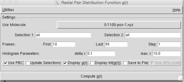
Using the “radial distribution function” plugin from the extension menu (Extensions>Analysis>Radial Pair Distribution Function g( r ) ), draw the g( r ) of the system.

Assignments:

Discuss radial distribution function for 700, 1100, and 1300 K.

Hint: how to use the g( r ) module:

First apply pbcs (see above)
Open the radial distribution function plugin and enter the parameters as shown (note: in the example below we excluded the first 10 frames) (from “Utilities” you can check that your unit cell is OK)
Click “Compute g( r )”
From the “File” menu of the graph window, you can save as postscript file or other formats.