
38 atom Lennard-Jones cluster: molecular dynamics with python
In this exercise you will perform molecular dynamics with a python program that you may inspect and modify directly. Then, you will perform the same kind of dynamics using cp2k and compare the performance.
you@eulerX ~$ wget http://www.cp2k.org/_media/exercises:2017_ethz_mmm:e2_bis.zip
you@eulerX ~$ unzip exercises:2017_ethz_mmm:e2_bis.zip
you@eulerX ~$ cd exercise_2
> cd
> nano .bashrc
module load new gcc/4.8.2 python/2.7.12 # include this line in the file
> . .bashrc
To visualize an xyz file:
> ipython

In [1]: from ase.io import read
In [2]: from ase.visualize import view
In [3]: s=read("file.xyz")
In [4]: view(s)
At this point you can rotate the structure, select an atom, then two (you get the distance) or three (you get the angle)…
In the repository you will find the program “md.py” and the geometry file “fcc_r.xyz” The program md.py can perform a MD simulation for a system of Ar atoms interacting via Lennard-Jones potential.
Executing the command
>python md.py
the program will ask you to provide
- the name of a geometry file
- the timestep to be used for the simulation in [fs]
- the total number of steps of dynamics to be performed
- the initial temperature desired for the system in [K]
At this point a window like that should open:
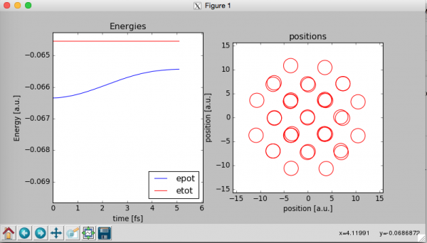
The program will show two graphs wile the MD simulation is running. The graph on the left contains the total energy of the system Etot that should remain constant along the simulation and the potential energy of the system “Epot”. Etot=Epot+Ekin where Ekin is the kinetic energy of the system.
At the end of execution the plot will be saved in the working directory as plots.png. You can visualize it by giving the command
> display plots.png
and data for the energy and temperature at each step will be saved on the file data.out. You can visualize the graphs using gnuplot: for the time vs. temperature:
> gnuplot
    gnuplot> plot 'data.out' u 2:7 w l
- 0.5 as timestep
- 1000 as total number of steps
- 20 as initial temperature for the system
Is the total energy conserved? Is the temperature of the system conserved?
- TASK 2 Execute the program with input parameters
- 1.8 as timestep
- 1000 as total number of steps
- 80 as initial temperature for the system
Is the total energy conserved?
Copy the program md.py into md_original.py and edit the file md.py (using nano). Have a look at the structure of the program At the beginning two functions are defined:
ekin(m,v) needs as input the mass of each atom and its velocity; computes the kinetic energy of the system.
forces_pot(pos,sigma,epsilon) needs as input the positions and the Lennard-Jones parameters to compute the potential energy of the system and the force on each atom. Then the program will:
- define the input parameters
- define atomic units and convert input data into atomic units
- initialize randomly velocities and rescale them to the desired initial temperature *
- define variables used for the graphs
Finally the main loop of the dynamics starts, and it contains a final block needed to produce the graphs.
Have a look at the function to compute the forces and the potential energy. A potentially very slow version of the algorithm is commented “#” (it would be very slow in an efficient fortran or C code that is compiled without optimization). The active version of the algorithm is supposed to be faster. Deactivate printing of data and production of the graphs by setting to False the two variables
execute three or four times the program and write down the execution time that you get as the only output. Now comment the lines for the “efficient” algorithm and uncomment the lines of the ”unefficient” one. Execute 3-4 times. Is the execution time longer? Why do you think you get such a result?
Find the section of the code that removes the initial linear momentum. What could you do to remove the initial angular momentum? (no need to write down the code, just think how you could do)
Molecular dynamics using CP2K
In this second part of the exercise, the same kind of dynamics will be performed with cp2k. You will find in the repository (zip file) the input file md.inp, where the &MOTION section is different from the last lecture exercise.
&MOTION
  &PRINT
    &RESTART_HISTORY OFF
    &END
    &RESTART
      &EACH
        MD 5000
      &END
    &END
    &TRAJECTORY
      &EACH
        MD 100
      &END
    &END
  &END
  &MD
    ENSEMBLE NVE
    STEPS 10000
    TIMESTEP 0.5
    TEMPERATURE 10.0
  &END MD
&END MOTION
> cp2k.popt -i md.inp > md.out
Compare the performance with the one of the python code. What do you notice? Plot the energy by using the file MD-1.ener and gnuplot
- What is the value of the total energy? Is it conserved?
- Increase the time step to 3 fs, and run it again. What happens to the total energy?
- Note: to visualize a trajectory you can use the code (look inside it!) traj.py in the directory:
python traj.py