In this exercise we will study the $S_N2$ nucleophilic substitution reaction

$$ \text{Cl}^- + \text{CH}_3\text{Cl} \longleftrightarrow \text{Cl}\text{CH}_3 + \text{Cl}^-. $$

For energy and force evaluation, we will use the Parameterization Method 6 (PM6), which is a relatively inexpensive semiempirical model for electronic structure evaluation. For accurate reaction characterizations, ab initio methods, such as DFT or higher level, should be used.

In order to find the activation barrier for the reaction we will use the NEB method. The NEB method provides a way to find the minimum energy path (MEP) between two different conformations of the system corresponding local potential energy minima. The MEP is a one-dimensional path on the $3N$-dimensional potential energy landscape and every point on the MEP is a potential energy minimum in all directions perpendicular to the path. MEP passes at least one saddle point and the energy of the highest saddle point is the peak of the activation barrier of the reaction.

To start the NEB calculation, we first need two different geometries at local energy minima, which we can obtain by running geometry optimization calculations. Use the following CP2K input script to obtain the first geometry:

geo.inp

&GLOBAL
  PRINT_LEVEL LOW
  PROJECT ch3cl
  RUN_TYPE GEO_OPT                # Geometry optimization calculation
&END GLOBAL

&MOTION
  &GEO_OPT                        # Parameters for GEO_OPT convergence
    MAX_FORCE 1.0E-4
    MAX_ITER 2000
    OPTIMIZER BFGS
    &BFGS
      TRUST_RADIUS [bohr] 0.1
    &END
  &END GEO_OPT
&END MOTION

&FORCE_EVAL
  METHOD Quickstep                # Quickstep - Electronic structure methods
  &DFT
   CHARGE -1                      # There is a negatively charged anion
    &QS
      METHOD PM6                  # Parametrization Method 6
      &SE
      &END SE
    &END QS
    &SCF                          # Convergence parameters for force evaluation
      SCF_GUESS ATOMIC
      EPS_SCF 1.0E-5
      MAX_SCF 50
       &OUTER_SCF
          EPS_SCF 1.0E-7
          MAX_SCF 500
       &END
    &END SCF
    &POISSON                      # POISSON solver for non-periodic calculation
      PERIODIC NONE
      PSOLVER WAVELET
    &END
  &END DFT

  &SUBSYS
    &CELL
      ABC 10.0 10.0 10.0
      PERIODIC NONE
    &END CELL
    &COORD
C      -4.03963494       0.97427857      -0.29785096
H      -3.97152206       2.11080568      -0.35500445
H      -3.95108814       0.19729141       0.53163699
H      -3.95810737       0.47922964      -1.32151084
Cl     -5.77885435       1.07089312      -0.04609427
Cl     -1.77974793       0.99422072      -0.29785096
    &END COORD
   &END SUBSYS
&END FORCE_EVAL

Now we are ready to start the NEB. Obtain the two optimized geometries from the GEO_OPT trajectories (last step in the ch3cl-pos-1.xyz file) to a separate folder and name them init.xyz and final.xyz. Now the NEB calculation can be run by the following input script:

neb.inp

&GLOBAL
  PRINT_LEVEL LOW
  PROJECT ch3cl
  RUN_TYPE BAND                      # Nudged elastic band calculation
&END GLOBAL

&MOTION
  &BAND
    NUMBER_OF_REPLICA 10             # Number of "replica" geometries along the path
    K_SPRING 0.05
    &OPTIMIZE_BAND
      OPT_TYPE DIIS
      &DIIS
        MAX_STEPS 1000
      &END
    &END
    BAND_TYPE CI-NEB                 # Climbing-image NEB
    &CI_NEB
      NSTEPS_IT  5                   # First take 5 normal steps, then start CI
    &END
    &REPLICA
      COORD_FILE_NAME init.xyz
    &END
    &REPLICA
      COORD_FILE_NAME final.xyz
    &END
    &PROGRAM_RUN_INFO
     INITIAL_CONFIGURATION_INFO
    &END
  &END BAND
&END MOTION

&FORCE_EVAL
  METHOD Quickstep
  &DFT
    ... same as GEO_OPT ...
  &END DFT
  &SUBSYS
    &CELL
      ABC 10.0 10.0 10.0
      PERIODIC NONE
    &END CELL
    &TOPOLOGY
      COORD_FILE_NAME init.xyz
      COORDINATE xyz
    &END TOPOLOGY
  &END SUBSYS
&END FORCE_EVAL

In the main output of the NEB calculation, you will find a number of the following sections:

*******************************************************************************
 BAND TYPE                     =                                          CI-NEB
 BAND TYPE OPTIMIZATION        =                                              SD
 STEP NUMBER                   =                                               1
 NUMBER OF NEB REPLICA         =                                              10
 DISTANCES REP =        0.252266        0.229810        0.225933        0.227113
                        0.201788        0.138731        0.138676        0.204817
                        0.252328
 ENERGIES [au] =      -24.815004      -24.813368      -24.808500      -24.803002
                      -24.800607      -24.802583      -24.805589      -24.809114
                      -24.813372      -24.815004
 BAND TOTAL ENERGY [au]        =                             -248.08548199708440
 *******************************************************************************

These sections show for every replica geometry along the NEB trajectory, the distance to its neighbors and its energy. The final section corresponds to the converged NEB trajectory.

Sampling the free energy surface (FES) of a chemical system is a convenient method to explore various stable conformations and possible reaction pathways. To calculate the FES for complicated systems, advanced sampling methods (such as umbrella sampling, metadynamics, parallel tempering, …) have to be used. However, for our simple $S_N2$ reaction, we will use unbiased Molecular Dynamics (MD).

The FES is a projection of the high-dimensional free energy landscape into a small number, usually two, dimensions. These two dimensions are called collective variables (CV) and they must be chosen such that various stable conformations can be distinguished and the reaction pathways can be adequately described by the FES. For complex systems, the choice of CVs is a non-trivial task. Fortunately for our simple system, the choice is simple: we take the distances of the two Cl anions from the central C as the CVs.

To help the calculation sample the parts of FES we care about, we will include restraints in the MD run, which prevent the Cl anions from going too far from the molecule.

The following CP2K input script runs our MD calculation and prints out the CV values for every step:

md.inp

&GLOBAL
  PRINT_LEVEL LOW
  PROJECT ch3f
  RUN_TYPE MD                 # Molecular Dynamics
&END GLOBAL
&MOTION
  &MD                         # MD parameters
    ENSEMBLE NVT
    STEPS 200000
    TIMESTEP 0.5
    TEMPERATURE 1000.0
    &THERMOSTAT
      TYPE NOSE
      &NOSE
        TIMECON 100.
      &END NOSE
    &END THERMOSTAT
  &END MD
  &CONSTRAINT                 # Restraints to keep Cl from going too far
    &COLLECTIVE
      INTERMOLECULAR
      COLVAR 1
      TARGET 1.8
      &RESTRAINT
        K 0.005
      &END
    &END
    &COLLECTIVE
      INTERMOLECULAR
      COLVAR 2
      TARGET 1.8
      &RESTRAINT
        K 0.005
      &END
    &END
  &END

  &FREE_ENERGY                 # Section to print out the values of CVs every step
    &METADYN
      DO_HILLS .FALSE.
      &METAVAR
        SCALE 0.2
        COLVAR 1
      &END
      &METAVAR
        SCALE 0.2
        COLVAR 2
      &END
      &PRINT
        &COLVAR
          COMMON_ITERATION_LEVELS 3
          &EACH
            MD 1
          &END
        &END COLVAR
      &END PRINT
    &END METADYN
  &END FREE_ENERGY
&END MOTION

&FORCE_EVAL
  METHOD Quickstep
  &DFT
   ... Same as before ...
  &END DFT

  &SUBSYS
    &CELL
      ABC 10.0 10.0 10.0
      PERIODIC NONE
    &END CELL
    &COORD
C      -4.03963494       0.97427857      -0.29785096
H      -3.97152206       2.11080568      -0.35500445
H      -3.95108814       0.19729141       0.53163699
H      -3.95810737       0.47922964      -1.32151084
Cl     -5.77885435       1.07089312      -0.04609427
Cl     -1.77974793       0.99422072      -0.29785096
    &END COORD

    &COLVAR                    # CV definitions
      &DISTANCE
        ATOMS 1 5
      &END
    &END COLVAR
    &COLVAR
      &DISTANCE
        ATOMS 1 6
      &END
    &END COLVAR
   &END SUBSYS
&END FORCE_EVAL

Free energy is expressed by

$$ F(s) = -k T \log(P(s)),$$

where $s$ is the set CVs and $P(s)$ is the probability that the system has the set of CV values $s$.

The following Python script can be used to calculate the FES from the ch3f-COLVAR.metadynLog file produced by the MD run. (Don't forget to change the temperature in Python script!)

import numpy as np
import matplotlib.pyplot as plt
import ase

bohr_2_angstrom = 0.529177
kb = 8.6173303e-5 # eV * K^-1

temperature = 1000.0                          #Change temperature according to your MD simulations!
colvar_path = "./ch3f-COLVAR.metadynLog"

# Load the colvar file
colvar_raw = np.loadtxt(colvar_path)

# Extract the two CVs
d1 = colvar_raw[:, 1] * bohr_2_angstrom
d2 = colvar_raw[:, 2] * bohr_2_angstrom

# Create a 2d histogram corresponding to the CV occurances
cv_hist = np.histogram2d(d1, d2, bins=50)

# probability from the histogram
prob = cv_hist[0]/len(d1)

# Free energy surface
fes = -kb * temperature * np.log(prob)

# Save the image
extent = (np.min(cv_hist[1]), np.max(cv_hist[1]), np.min(cv_hist[2]), np.max(cv_hist[2]))
plt.figure(figsize=(8, 8))
plt.imshow(fes.T, extent=extent, aspect='auto', origin='lower', cmap='hsv')
cbar = plt.colorbar()
cbar.set_label("Free energy [eV]")
plt.xlabel("d1 [ang]")
plt.ylabel("d2 [ang]")
plt.savefig("./fes.png", dpi=200)
plt.close()

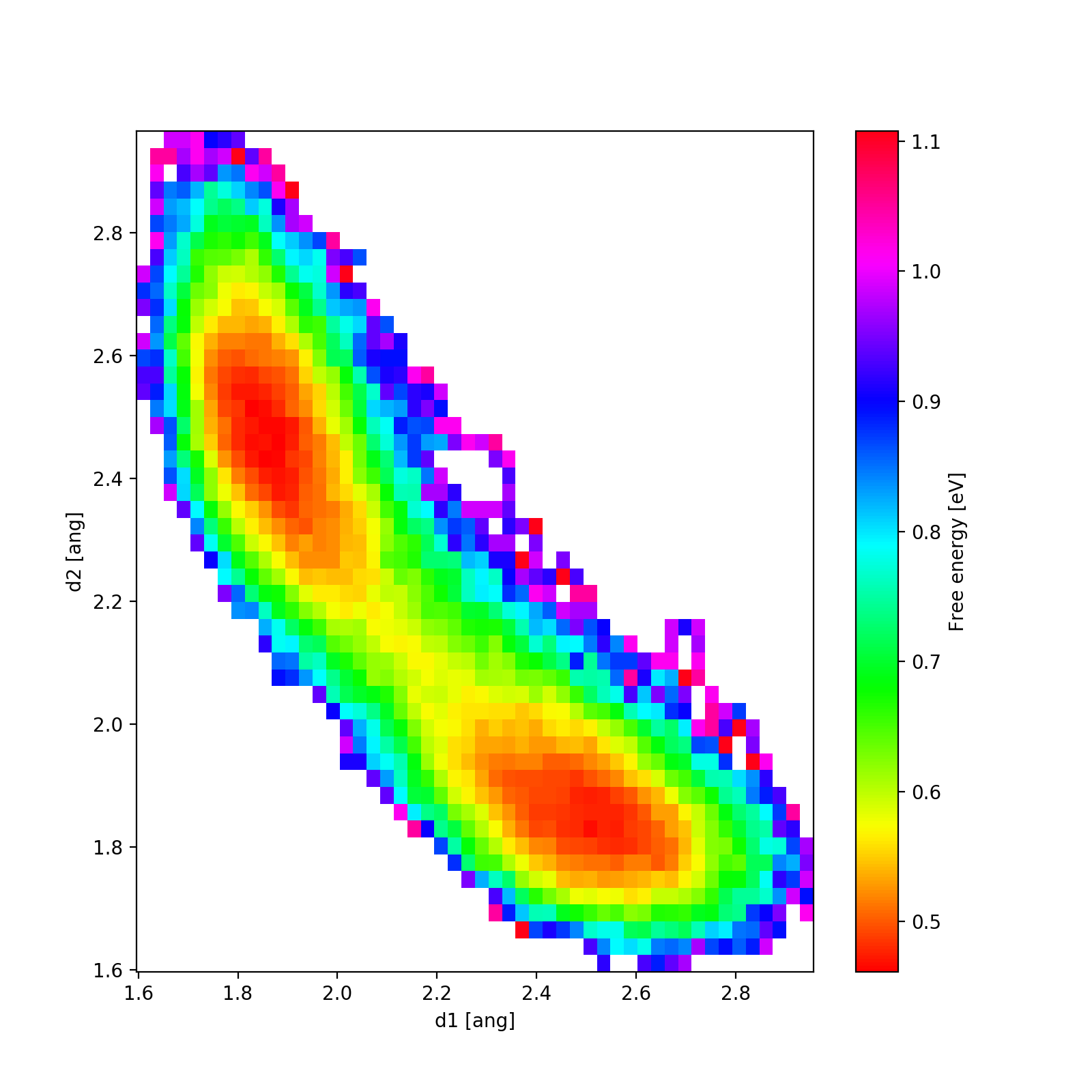
Here is an example output for temperature 1000K. We clearly see the two local minima corresponding to the one of the chlorine atoms being covalently bonded (distance 1.8 Å) while the other one is around distance 2.5 Å.