Simple STM images

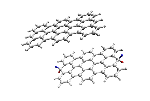
In this exercise we will consider different termination of two polyantryl molecules that are an intermediate step for the formation of a long armchair nanoribbon. 10.1021/ja311099k.

We will show how a simple change in the termination (1 vs. 2 Hydrogens) changes the state structure completely.

You should run these calculations on 16 nodes with bsub -n 16. Download, as usual, the files from the media manager: exercise_10.2.tar.gz. The 1h.1.5.inp file is commented).

1. Task: Running the job and looking at the orbitals

This time we will not optimize the structure. With an ENERGY run, we run with cp2k the job 1h.1.5.inp and 2h.1.5.inp, meaning that there are here 1.5 units of the original molecule in the gas phase.

The interesting part of the code is in the &PRINT section of &DFT :

    &PRINT
! controls the printing of cubes for the generation of STM images.
    &STM
! set of sample bias
! negative for occupied states and positive for unoccupied states
      BIAS -2.0 -1.0 1.0 2.0
! orbital symmetry of the tip
! The change in the tip symmetry can radically alter the contrast of the topographic
! image due to changes in tip-surface overlap
      TH_TORB S
    &END STM
! print molecular orbitals
    &MO_CUBES
! 10 occupied orbitals
       NHOMO 10
! 10 unoccupied orbitals
       NLUMO 10
! limit the size of cube files
       STRIDE 2 2 2
       WRITE_CUBE T
    &END
! a cube file with eletrostatic potential generated by the total density (electrons+ions).
    &V_HARTREE_CUBE
    &END

      &MO
! molecular orbitals eigenvalues and molecular ocuupations after each scf
       FILENAME EIG
! add the last iteration with description
       ADD_LAST NUMERIC
! printing of eigenvalues of molecular orbitals
       EIGENVALUES
! also print occupation of the molecular orbitals
       OCCUPATION_NUMBERS
      &END
    &END

There will be an output file with the energy levels and their occupation. The last one can be easily found…

Hitting ls -ltr will allow you to see on the last lines of the screen the most recent files.

Draw the energy level diagram for the two molecules. What is the energy gap in the two cases? What are the differences?
Look with vmd at the cube files corresponding to the most interesting levels (close to Fermi…). Comment on the distribution of the states.

2. Task: Producing a simple STM image

The section &STM shown above produces STM images at different bias (feel free to change), meaning, using the Tersoff-Hamann approximation, it integrates all the density of states with energies between Fermi energy and the Bias potential: this energy interval is involved in the tunnel current. The *STM*cube files are 3D maps of the integrated density of states. Imagine that we have a microscope with a feedback that can keep constant current between tip and sample, by changing the height of the tip on the surface. Since the current is proportional to the density of states, we move the tip on isosurfaces of our cubefile. The program stm ** (in the same working dir) allows to extract a 2D map of the height of a given isosurface.

Run the program in the following way:
$ module load boost/1.54.0
$ module load mkl
$ stm -c 2h*STM*.cube --isovalues 1E-5 > stm.out

The resulting .igor files contain the z profile (in bohr) and may for example be plotted by gnuplot:

gnuplot
set pm3d map
set size square
set xrange [......
set yrange [.....

splot "mystm.igor" matrix using 2:1:3

Where instead of “mystm” you use an appropriate filename.

In the output file of cp2k, the program tells you how many states have contributed to each STM image. Discuss the images that you see in the two cases.
What makes the 1h* case particular with respect to the 2h*?
Change the isosurface and look at the z-range. Discuss the changes in the range.
Would you define the differences between 1h and 2h in the STM images as more of structural origin or electronic origin?