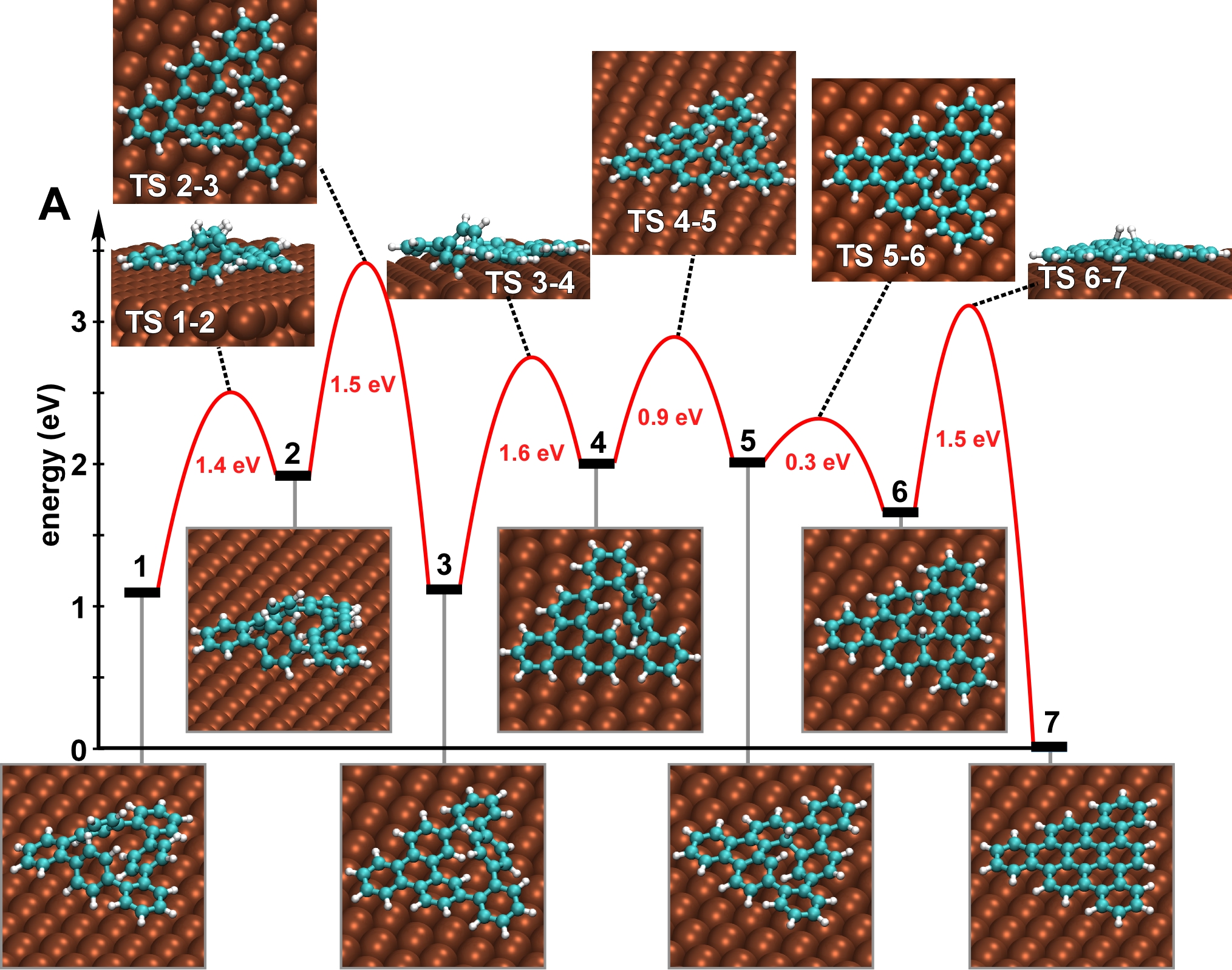
Problem: compute activation barrier for the last step (6 to 7) of the cyclodehydrogenation reaction CHP@Cu(111) → TBC

• Original author: Carlo Pignedoli
• Complete source and output files: NEB.tar.xz

The system is composed by a molecule (56 atoms) adsorbed on a Cu(111) slab (~2900 atoms). The molecule is treated within DFT (PM6¹⁾ in the exercise) and the substrate with EAM²⁾ potentials. The substrate and the molecule are coupled through a par potential mimicking the van der Waals interaction and Pauli repulsion.³⁾

We need MULTIPLE_FORCE_EVALS:

• In a first section we define how to partition the whole system in a DFT+EMPIRICAL part
• in a second section we define the force fields for the EMPIRICAL part
• and in the third section we define the parameters for the DFT part.
• The fourth and final section defines the target of the calculation(GEO_OPT, NEB, Molecular dynamics..)

The files for this part of the exercise are found in the EX2 folder.

Here we specify that our system consists of two fragments: atoms 1 to 56 and atoms 57 to 2936, the whole system is contained in the cell specified in FORCE_EVAL/SUBSYS section.

We declare that the first FORCE_EVAL section following the present one will be dedicated to FRAGMENTS 1 and 2 (it will contain the empirical potentials) and the second FORCE_EVAL section will be devoted to FRAGMENT 1 only (the DFT treatment of the molecule).

&MULTIPLE_FORCE_EVALS
  FORCE_EVAL_ORDER 2 3
  MULTIPLE_SUBSYS T
&END
&FORCE_EVAL
  METHOD MIXED
  &MIXED
    MIXING_TYPE GENMIX
    GROUP_PARTITION 1 1
    &GENERIC
      ERROR_LIMIT 1.0E-10
      MIXING_FUNCTION E1+E2
      VARIABLES E1 E2
    &END
    &MAPPING
       &FORCE_EVAL_MIXED
         &FRAGMENT 1
            1 56
         &END
         &FRAGMENT 2
            57 2936
         &END
       &END
       &FORCE_EVAL 1
         DEFINE_FRAGMENTS 1 2
       &END
       &FORCE_EVAL 2
         DEFINE_FRAGMENTS 1
       &END
    &END
  &END
  &SUBSYS
   &COLVAR
    &DISTANCE
     ATOMS 49 50
    &END
   &END
    &CELL
      ABC  40.764229 39.715716 70.
    &END CELL
    &TOPOLOGY
      COORD_FILE_NAME ./s.xyz
      COORDINATE XYZ
      CONNECTIVITY OFF
    &END TOPOLOGY
  &END SUBSYS
&END

In this section we define the empirical potentials for the whole system: EAM will be used for the Cu-Cu interactions (parametrized in the file Files/CU.pot), a C6/R^6 + pauli repulsion will be defined for C-Cu and H-Cu and, finally, NULL interactions will be defined for C-C, C-H and H-H since these will be obtained from DFT in the next section. The charge of every specie (zero in our example) as well as the interaction within each possible type-pair has to be defined.

&FORCE_EVAL
  METHOD FIST
  &MM
   &FORCEFIELD
     &SPLINE
       EPS_SPLINE 1.0E-6
       EMAX_SPLINE 0.9
     &END
     &CHARGE
       ATOM Cu
       CHARGE 0.0
     &END CHARGE
     &CHARGE
       ATOM H
       CHARGE 0.0
     &END CHARGE
     &CHARGE
       ATOM C
       CHARGE 0.0
     &END CHARGE
     &NONBONDED
       &GENPOT
          atoms Cu C
          FUNCTION A*exp(-av*r)+B*exp(-ac*r)-C/(r^6)
          VARIABLES r
          PARAMETERS A av B ac C
          VALUES 4.13643 1.33747 115.82004 2.206825 75.40708524085266692113
          RCUT  15
       &END GENPOT
       &GENPOT
          atoms Cu H
          FUNCTION A*exp(-av*r)+B*exp(-ac*r)-C/(r^6)
          VARIABLES r
          PARAMETERS A av B ac C
          VALUES 0.878363 1.33747 24.594164 2.206825 21.32834305207502214234
          RCUT 15
       &END GENPOT
       &LENNARD-JONES
         atoms C H
         EPSILON 0.0
         SIGMA 3.166
         RCUT  15
       &END LENNARD-JONES
        &LENNARD-JONES
         atoms H H
         EPSILON 0.0
         SIGMA 3.166
         RCUT 15
       &END LENNARD-JONES
       &LENNARD-JONES
         atoms C C
         EPSILON 0.0
         SIGMA 3.166
         RCUT 15
       &END LENNARD-JONES
       &EAM
         atoms Cu Cu
         PARM_FILE_NAME ../../Files/CU.pot
       &END EAM
     &END NONBONDED
   &END FORCEFIELD
   &POISSON
     &EWALD
       EWALD_TYPE none
     &END EWALD
   &END POISSON
  &END
  &SUBSYS
    &CELL
      ABC  40.764229 39.715716 70.
    &END CELL
    &TOPOLOGY
      COORD_FILE_NAME ./s.xyz
      COORDINATE XYZ
      CONNECTIVITY OFF
    &END TOPOLOGY
  &END SUBSYS
&END

In this section we specify the parameters for the DFT treatment of the molecule. Note that the simulation cell here is reduced with comparison to the simulation cell of the whole system.

&FORCE_EVAL
  METHOD Quickstep
  &DFT
    &QS
      METHOD PM6
      EXTRAPOLATION USE_GUESS
      &SE
        &COULOMB
          CUTOFF [angstrom] 20.0
        &END
        &EXCHANGE
          CUTOFF [angstrom] 20.0
        &END
      &END
    &END QS
    &SCF
      MAX_SCF 20
      SCF_GUESS RESTART
      EPS_SCF 1.0E-6
      &OT
        PRECONDITIONER  FULL_SINGLE_INVERSE
        MINIMIZER DIIS
        N_DIIS 7
      &END
      &OUTER_SCF
        MAX_SCF 10
        EPS_SCF 1.0E-6
      &END
      &PRINT
        &RESTART
          &EACH
            QS_SCF 0
          &END
          ADD_LAST NUMERIC
        &END
        &RESTART_HISTORY OFF
        &END
      &END
    &END SCF
    &POISSON
      PERIODIC NONE
      POISSON_SOLVER WAVELET
      &WAVELET
        SCF_TYPE 60
      &END
    &END POISSON
    &XC
      &XC_FUNCTIONAL BLYP
      &END XC_FUNCTIONAL
    &END XC
!   &PRINT
!     &MO_CUBES
!       NHOMO 15
!       NLUMO 15
!       WRITE_CUBE T
!       LOG_PRINT_KEY
!     &END
!   &END
  &END DFT
  &SUBSYS
    &CELL
      ABC  30 30 30
      PERIODIC NONE
    &END CELL
    &TOPOLOGY
      COORD_FILE_NAME ./f.xyz
      COORDINATE xyz
      &CENTER_COORDINATES
      &END
    &END
#    &KIND H
#      BASIS_SET TZV2P-MOLOPT-GTH
#      POTENTIAL GTH-BLYP-q1
#    &END KIND
#    &KIND C
#      BASIS_SET TZV2P-MOLOPT-GTH
#      POTENTIAL GTH-BLYP-q4
#    &END KIND
  &END SUBSYS
&END FORCE_EVAL

In this section we define the target of the simulation as a geometry optimization this will be MD, or BAND in other examples.

&GLOBAL
  PRINT_LEVEL LOW
  PROJECT INI
  RUN_TYPE GEO_OPT
  WALLTIME 28000
&END GLOBAL
&MOTION
 &GEO_OPT
    MAX_FORCE 0.0001
    MAX_ITER 500
    OPTIMIZER LBFGS
    &LBFGS
    &END
 &END
&END
!&EXT_RESTART
!  RESTART_FILE_NAME constr_3cc_2h_41_dft-1.restart
!&END

1. First of all obtain the equilibrium geometry for the initial and the final states (in the directories INI and FIN you will find the input files (INI/geo.inp/FIN/geo.inp) the output files (INI/out/FIN/out) and the trajectory of the geometry optimization (INI-pos-1.xyz and FIN-pos-1.xyz).
   1. Please note that the geometry optimization of the final state is constrained with respect to the position of the final H2 molecule.
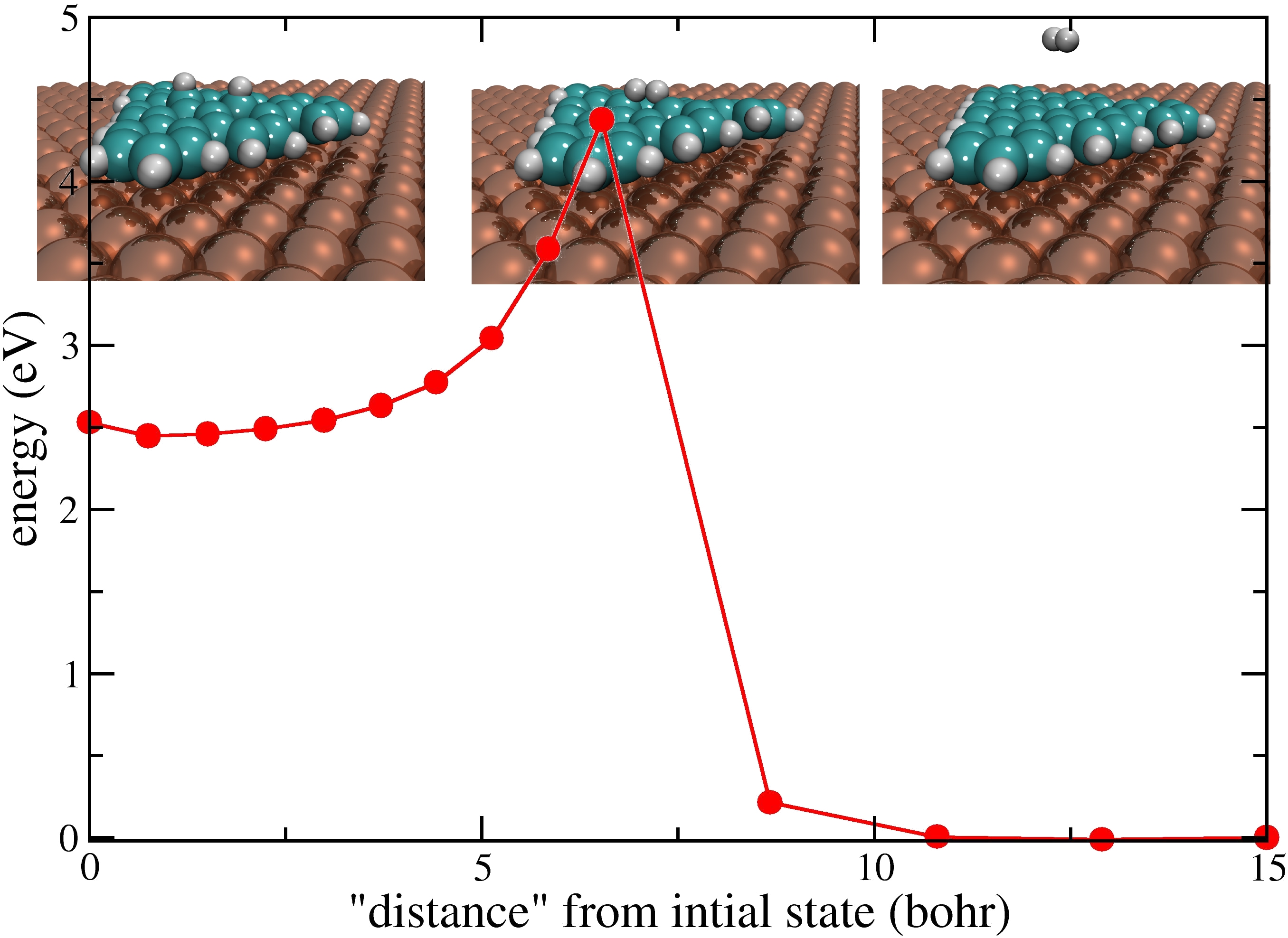
2. Perform a NEB simulation to find a saddle point between ini_eq.xyz and fin_eq.xzy.
   1. A linear guess for the path is not a good idea in this case; a clever guess can be obtained from a series of constrained geometry optimizations where the H-H distance is forced to vary from its initial value (more than 3 Å) to the H2 equilibrium distance. Such a guess is given, in the directory EX2, with the files ini_eq.xyz, due.xyz,tre.xyz,…,tredici.xyz,fin_eq.xyz).
      Check that the initial step of the NEB calculation is reasonable and determine the activation barrier at the and of the optimization. In the directory EX2 you will find the input for the calculation (neb.inp), the output (out) and the optimization trajectory of each image of the system (NEB-pos-Replica_nr_XX-1.xyz, 14 images are used in the example)

The last section of the input described above is modified as follows:

&GLOBAL
  PRINT_LEVEL LOW
  PROJECT NEB
  RUN_TYPE BAND
  WALLTIME 28000
&END GLOBAL
&MOTION
  &BAND
    NPROC_REP 2
    BAND_TYPE CI-NEB
    NUMBER_OF_REPLICA 14
    K_SPRING 0.05
    &CONVERGENCE_CONTROL
      MAX_FORCE 0.0030
      RMS_FORCE 0.0050
      MAX_DR 0.002
      RMS_DR 0.005
    &END
    ROTATE_FRAMES F
    ALIGN_FRAMES F
    &CI_NEB
       NSTEPS_IT  2
    &END
    &OPTIMIZE_BAND
      OPT_TYPE DIIS
      OPTIMIZE_END_POINTS F
      &DIIS
        MAX_STEPS 1000
      &END
    &END
#
    &REPLICA
      COORD_FILE_NAME  ini_eq.xyz
    &END

    &REPLICA
      COORD_FILE_NAME  due.xyz
    &END
.
.
.
.
.
    &REPLICA
      COORD_FILE_NAME  fin_eq.xyz
    &END

    &PROGRAM_RUN_INFO
     INITIAL_CONFIGURATION_INFO
    &END
    &CONVERGENCE_INFO
    &END
 &END
&END

We declare that we need 14 replicas and each replica has to be computed with 2 CPUS (if we run the calculation with 14 cpus, then every group of 2 cpus will work on two replicas). The initial guess for the reaction path is given through 14 geometry files.

The files for this part of the exercise are found in the EX1 folder.

Obtain two restart files for independent configurations of the system at the geometry of the initial state thermalized at 450 K. In the directory EQUIL the input file inp is used to run 3000 MD steps of MD in the NVT ensamble with a CSVR thermostat (a longer simulation should be used) two restart files obtained during the simulation (EQUIL-1_2000.restart and EQUIL-1_3000.restart) will be used to run a Metadynamics simulation with two WALKERS. The trajectory of the MD should be also used to define the shape of the gaussians added in the metadynamics run. Trajectories are printed in dcd format (EQUIL-pos-1.dcd use, e.g. vmd s.xyz EQUIL-pos-1.dcd to visualize the trajectory).

The MOTION section will look like:

&MOTION
  &MD
    ENSEMBLE NVT
    STEPS    3000
    TIMESTEP 0.5
    TEMPERATURE 450.0
    &THERMOSTAT
       TYPE CSVR
       REGION MASSIVE
       &CSVR
          TIMECON [fs] 200.0
       &END
    &END
  &END MD
  &PRINT
    &TRAJECTORY
      FORMAT DCD
      &EACH
        MD 100
      &END
    &END
    &RESTART
      &EACH
        MD 1000
      &END
      FILENAME EQUIL
    &END
    &RESTART_HISTORY
     &EACH
      MD 1000
     &END
    &END
  &END
&END

The two restart files are copied in the directory Files (r1 and r2 respectively). In the directory also the geometry for the whole system in the initial configuration as well as the geometry of the molecular fragment are included (files s and f respectively).

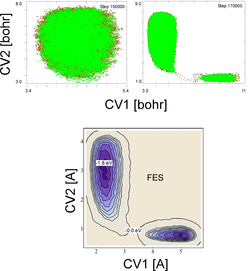
We perform a metadynamics simulation with two collective variables: the sum of C-H distances (CV1) and the H-H distance (CV2). Walls have to be introduced to limit the range of variability of the two CVs.

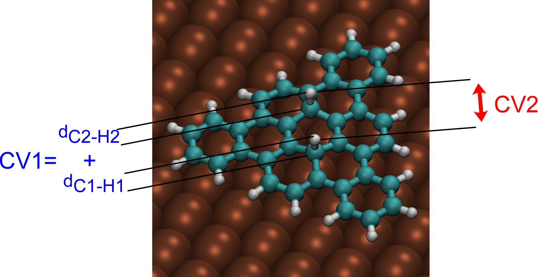
To define the collective variables introduce a COLVAR card in the SUBSYS section of the first FORCE_EVAL:

  &SUBSYS
    &COLVAR
       &COMBINE_COLVAR
          &COLVAR
             &DISTANCE
                ATOMS 4 50
             &END
          &END COLVAR
          &COLVAR
             &DISTANCE
                ATOMS 7 49
             &END
          &END COLVAR
          FUNCTION CV1+CV2
          VARIABLES CV1 CV2
          ERROR_LIMIT 1.0E-8
       &END
    &END
    &COLVAR
     &DISTANCE
      ATOMS 49 50
     &END
    &END

The MOTION section has to be modified as follows to activate metadynamics on the two CVs:

&MOTION
  &MD
    ENSEMBLE NVT
    STEPS    50000
    TIMESTEP 0.5
    TEMPERATURE 450.0
    &THERMOSTAT
       TYPE CSVR
       REGION MASSIVE
       &CSVR
          TIMECON [fs] 200.0
       &END
    &END
  &END MD
  &FREE_ENERGY
    &METADYN
      DO_HILLS
      NT_HILLS 50
      WW 2.0e-3
      &METAVAR
        SCALE 0.1
        COLVAR 1
        &WALL
          TYPE QUADRATIC
          POSITION [angstrom] 5
          &QUADRATIC
             DIRECTION WALL_PLUS
             K [kcalmol] 40.0
          &END
        &END
        &WALL
          TYPE QUADRATIC
          POSITION [angstrom] 1.90
          &QUADRATIC
             DIRECTION WALL_MINUS
             K [kcalmol] 40.0
          &END
        &END
      &END METAVAR
      &METAVAR
        SCALE 0.1
        COLVAR 2
        &WALL
          TYPE QUADRATIC
          POSITION [angstrom] 3.80
          &QUADRATIC
             DIRECTION WALL_PLUS
             K [kcalmol] 40.0
          &END
        &END
        &WALL
          TYPE QUADRATIC
          POSITION [angstrom] 0.75
          &QUADRATIC
             DIRECTION WALL_MINUS
             K [kcalmol] 40.0
          &END
        &END
      &END METAVAR
#     &METAVAR
#       SCALE 0.1
#       COLVAR 3
#       &WALL
#         TYPE QUADRATIC
#         POSITION [angstrom] 4.00
#         &QUADRATIC
#            DIRECTION WALL_PLUS
#            K [kcalmol] 40.0
#         &END
#       &END
#       &WALL
#         TYPE QUADRATIC
#         POSITION [angstrom] 1.30
#         &QUADRATIC
#            DIRECTION WALL_MINUS
#            K [kcalmol] 40.0
#         &END
#       &END
#     &END METAVAR
      &PRINT
        &COLVAR
         COMMON_ITERATION_LEVELS 4
        &END
      &END
      &MULTIPLE_WALKERS
        NUMBER_OF_WALKERS 2
        WALKER_ID 1
        WALKER_COMM_FREQUENCY 4
        &WALKERS_FILE_NAME
           ../WALK_DATA_FILES/WALKER_1.data
           ../WALK_DATA_FILES/WALKER_2.data
        &END
      &END
    &END METADYN
  &END
  &PRINT
    &TRAJECTORY
      FORMAT DCD
      &EACH
        MD 100
      &END
    &END
    &RESTART
      &EACH
        MD 100
      &END
      FILENAME META
    &END
    &VELOCITIES ON
      &EACH
        MD 5000
      &END
    &END
    &RESTART_HISTORY OFF
    &END
  &END
&END
&EXT_RESTART
 RESTART_FILE_NAME ../../Files/r1
&END

The section specific to the multiple walkers could be removed to run the simulation with a single walker:

      &MULTIPLE_WALKERS
        NUMBER_OF_WALKERS 2
        WALKER_ID 1
        WALKER_COMM_FREQUENCY 4
        &WALKERS_FILE_NAME
           ../WALK_DATA_FILES/WALKER_1.data
           ../WALK_DATA_FILES/WALKER_2.data
        &END
      &END

Here we declare that we are using two walkers, that the input belongs to the walker with ID 1, that the data relative to the different walkers are stored in the files contained in the directory WALK_DATA_FILES and that the history of the gaussian hills deposited by each walker should be exchanged every 4 hills deposited.

We need two independent directories (WALK1 and WALK2 in the example) belonging to each WALKER, each directory will contain an input in which the WALKER ID is modified (1 and 2).

The calculation will run as a FARMING: we need a common input that specifies that we are running two cp2k problems:

The input file for the calculation (inp in the directory EX1) will be:

&GLOBAL
  PROGRAM FARMING
  RUN_TYPE NONE
&END GLOBAL

&FARMING
  NGROUP 2
  &JOB
    DIRECTORY WALK1
    INPUT_FILE_NAME inp
  &END JOB
  &JOB
    DIRECTORY WALK2
    INPUT_FILE_NAME inp
  &END JOB
&END FARMING

We declare that the cpus used for the calculation belongs to two groups of calculations, one job has to run in the directory WALK1 according to the prescriptions contained in the input file WALK1/inp and a second job has to run in the directory WALK2 (using WALK2/inp).

If we run the calculation with 8 cpus, 4 will be devoted to the JOB in directory WALK1 and 4 to WALK2. Each group of 10 cpus will be then partitioned according to partition instruction contained in each inp file (GROUP_PARTITION 1 3).

During execution you can monitor the evolution of the CVs of each walker from the files META-COLVAR.metadynLog and META-COLVAR.metadynLog

e.g.

plot  'WALK1/META-COLVAR.metadynLog'   u 2:3 pt 7.0 ps 1.0 t "",\
      'WALK2/META-COLVAR.metadynLog'   u 2:3 pt 7.0 ps 1.0 t ""

You can reconstruct the free energy profile from a restart file with the command:

fes.popt -cp2k -mathlab -file META-META-1.restart -ndim 2 -ndw 1 2 -out fes_12.dat