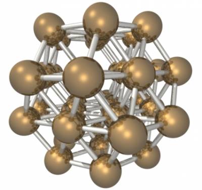
38 atom Lennard-Jones cluster

(picture by Luke Abraham)

TO USE THE FUNCTION LIBRARY (VERSION UP TO DATE) IN THE INTERACTIVE SHELL:

you@eulerX ~$ module load courses mmm vmd

you@eulerX ~$ mmm-init

REMEMBER: this is the command to load the module for the cp2k program:

you@eulerX ~$ module load cp2k

and to submit the job (note: since all the examples of this week are ultrafast, we will run them interactively, and NOT on a compute node. This is not the normal procedure for the next lectures).

you@eulerX ~$ cp2k.popt -i file.inp -o file.out

Download the 1.1 exercise into your $HOME folder and unzip it.

you@eulerX ~$ wget http://www.cp2k.org/_media/exercises:2017_ethz_mmm:exercise_1.1.zip
you@eulerX ~$ unzip exercises:2017_ethz_mmm:exercise_1.1.zip

All files of this exercise be downloaded from the wiki: exercise_1.1.zip

In this exercise you will test the Lennard-Jones potential. In particular, we will focus on the system described in the following paper about the energy landscape of the 38 atom Lennard-Jones cluster:

10.1063/1.478595

Login to euler using your nethz credentials. Then go to the directory “exercise_1.1”.

you@eulerX ~$ cd exercise_1.1

Geometry optimization

In this first part you will perform a simple energy optimization, to find the two lowest lying minima in the potential energy surface.

The input file structure of the template is the following:

geo_opt.inp

&GLOBAL
 FLUSH_SHOULD_FLUSH
 PRINT_LEVEL low
 PROJECT geo_opt_bfgs
 RUN_TYPE geo_opt
 WALLTIME 600
&END GLOBAL

&MOTION
 &GEO_OPT
  OPTIMIZER BFGS
  MAX_ITER  200
  MAX_DR    0.001
  RMS_DR    0.0003
  MAX_FORCE 0.0001
  RMS_FORCE 0.00003
  &BFGS
   USE_MODEL_HESSIAN yes
  &END BFGS
 &END GEO_OPT
 &PRINT
  &TRAJECTORY on
   FORMAT xyz
   &EACH
    GEO_OPT 1
   &END EACH
  &END TRAJECTORY
 &END PRINT
&END MOTION

&FORCE_EVAL
 METHOD Fist
 STRESS_TENSOR ANALYTICAL
 &MM
    &FORCEFIELD
      &CHARGE
        ATOM Ar
        CHARGE 0.0
      &END
      &NONBONDED
        &LENNARD-JONES
          atoms Ar Ar
          EPSILON 119.8
          SIGMA 3.405
          RCUT 8.4
        &END LENNARD-JONES
      &END NONBONDED
      &CHARGE
        ATOM Kr
        CHARGE 0.0
      &END CHARGE
    &END FORCEFIELD
  &POISSON
   PERIODIC NONE
   &EWALD
    EWALD_TYPE none
   &END EWALD
  &END POISSON
  &PRINT
   &FF_INFO OFF
    SPLINE_DATA
    SPLINE_INFO
   &END FF_INFO
  &END PRINT
 &END MM
 &PRINT
  &FORCES off
  &END FORCES
  &GRID_INFORMATION
  &END GRID_INFORMATION
  &PROGRAM_RUN_INFO
   &EACH
    GEO_OPT 1
   &END EACH
  &END PROGRAM_RUN_INFO
  &STRESS_TENSOR
   &EACH
    GEO_OPT 1
   &END EACH
  &END STRESS_TENSOR
 &END PRINT
 &SUBSYS
  &CELL
   A      100 0 0
   B      0   100 0
   C      0 0 100
   PERIODIC NONE
  &END CELL
  &TOPOLOGY
      COORD_FILE_NAME in.xyz
      COORDINATE xyz
  &END
  &PRINT
   &CELL
   &END CELL
   &KINDS
   &END KINDS
   &MOLECULES OFF
   &END MOLECULES
   &SYMMETRY
   &END SYMMETRY
  &END PRINT
 &END SUBSYS
&END FORCE_EVAL

NOTE ON THE UNITS: CP2K USES SO CALLED “atomic units”. Meaning that the resulting energies are expressed in Hartree, 1 Hartree=27.2114 eV. In the input file, the epsilon value (depth of the well) is expressed in KT units, namely, in “temperature” units (there is a Boltzmann constant to make units work…). The sigma value is in Angstrom.

load the module with the special m_* bash functions and initialize the module:
```
module load courses mmm ; mmm-init 
```
randomize the coordinate files fcc.xyz
```
m_xyzrand 1.0 < fcc.xyz > fcc_rand.xyz
```
. Do the same with ico.xyz
extract the q4 order parameter from fcc.xyz and from fcc_rand.xyz and compare the values.
```
module load new gcc/4.8.2 python/2.7.12  
python stein.py file.xyz 
```
. You will be asked the cutoff radius for the neighbors, it is 1.391 in sigma units. You should input it in Angstrom.
before running the simulation, copy the input coordinate file into in.xyz
```
cp fcc_rand.xyz in.xyz
```

run cp2k

module load cp2k

(this has only to be done once)

cp2k.popt -i geo_opt.inp -o geo_opt.out

in the output file, note the final energy, transform it in the unit of the paper (epsilon units)
load vmd module and play with the optimization trajectory
```
vmd OPT-pos-1.xyz
```
(ask the teacher)
apply the script myq4 to the optimization trajectory: this generates a list of q4 and energies for the whole trajectory.
```
./myq4 OPT-pos-1.xyz > fcc.ene.q4
```
plot q4 and energies with gnuplot (ask the teacher)
have a look at the myq4 script
```
nano myq4
```
repeat for the ico.xyz starting point, don't forget to first copy/remove the files appropriately. For example:
```
mkdir FCC ; mv OPT* FCC ; mv geo_opt.out FCC
```
finally, run the bash script
```
./curve
```
. Look inside, and try to understand what you get.

Assignment:

Report the energy of the minima, compare it with the ones of the initial configurations.
Plot q4 vs. energy and q4 vs. optimization steps, for the two cases. Discuss the results. Are the minima in two separate basins?
Report the value of the order parameter of the minumum, and discuss what you see
Use “gnuplot” to make the output of “./curve” understandable, discuss the results.