
Simple STM images
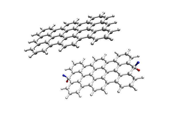
In this exercise we will consider different termination of two polyantryl molecules that are an intermediate step for the formation of a long armchair nanoribbon. 10.1021/ja311099k.
We will show how a simple change in the termination (1 vs. 2 Hydrogens) changes the state structure completely.
bsub -n 16.
Download, as usual, the files from the media manager: exercise-10.2.tar.gz. The 1h.1.5.inp file is commented).
Please use command module load cp2k/2.5.14075 , as well as module load python/2.7.9 to do this particular exercise.
1. Task: Running the job and looking at the orbitals
This time we will not optimize the structure. With an ENERGY run, we run with cp2k the job 1h.1.5.inp and 2h.1.5.inp. Here the number 1.5 represents the number of units of the original molecule in the gas phase.
The interesting part of the code is in the &PRINT section of &DFT :
    &PRINT
! controls the printing of cubes for the generation of STM images.
    &STM
! set of sample bias
! negative for occupied states and positive for unoccupied states
      BIAS -2.0 -1.0 1.0 2.0
! orbital symmetry of the tip
! The change in the tip symmetry can radically alter the contrast of the topographic
! image due to changes in tip-surface overlap
      TH_TORB S
    &END STM
! print molecular orbitals
    &MO_CUBES
! 10 occupied orbitals
       NHOMO 10
! 10 unoccupied orbitals
       NLUMO 10
! limit the size of cube files
       STRIDE 2 2 2
       WRITE_CUBE T
    &END
! a cube file with eletrostatic potential generated by the total density (electrons+ions).
    &V_HARTREE_CUBE
    &END
There will a lot of “EIG” files, but only the last (“EIG-1_0.MOLog”) file is of use for the energy level diagram plotting. Remove the other “EIG” files by using the command “ rm *EIG-1_0_*.MOLog”. To plot the energy level diagram, extract the energies from the eigenvalues file, and copy them (single column) into a file with the same shape as the provided example energy_ref.dat. Copy and paste following lines into the python script eldplot.py. The file energy_ref.dat contains the energy eigenvalues (in a.u.) in one column from the last “EIG” file (you can also use two names for the two molecules). The Fermi energy (Ef [a.u], is the energy of the highest occupied level) must be entered in the eldplot.py script. Use the command python eldplot.py to get the energy level diagram as a png image. (use display command to visualize it). Identify the occupied and unoccupied energy levels and name them. Feel free to change the png image name.
import matplotlib.pyplot as plt
import numpy as np
import scipy as spy
import pylab as ply
import argparse
import sys

# Open file

f = open('energy_ref.dat', 'r')

lines = f.readlines()

f.close()

x1 = []
y1 = []

# Fermi energy
Ef=0.0

for line in lines:
    p = map(float,line.split())
    y1.append(float((p[0]-Ef)*27.212))

for yv in y1:
    x = [0.2,0.8]
    y = [yv, yv]

    if yv <= 0:
        plt.plot(x,y,color='red')
    else:
        plt.plot(x,y,color='green')

# add label to y-axis
ply.ylabel("E - Ef [eV]")

# set x and y range
ply.xlim([0,1])
ply.ylim([-5,5])

# remove x-axis label
plt.gca().xaxis.set_major_locator(plt.NullLocator())

# show plot
#plt.show()

# save plot in a eps file
plt.savefig('ELD.png')
An example of the energy level diagram is as follows,
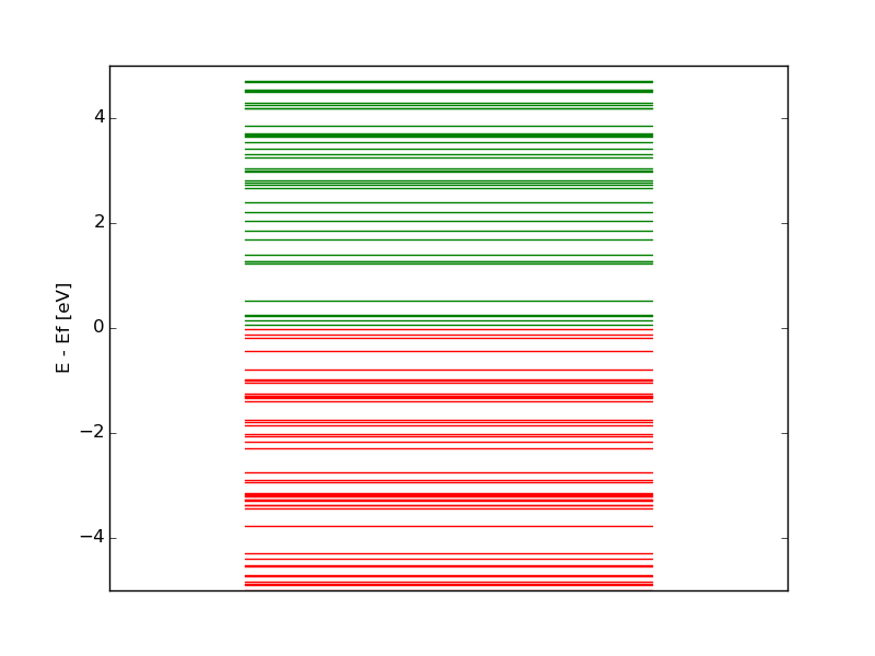
- Draw the energy level diagram for the two molecules. What is the energy gap in the two cases? What are the differences?
- Look with vmd the WFN cube files corresponding to the most interesting levels (close to the Fermi energy). Use command e.g. vmd -e orbitals.vmd 2H-WFN_00094_1-1_0.cube Comment on the distribution of the states.
2. Task: Producing a simple STM image
The section &STM shown above produces STM images at different bias voltages (feel free to change), meaning, using the Tersoff-Hamann approximation, it integrates all the density of states with energies between Fermi energy and the bias voltage: this energy interval is involved in the tunnel current. The *STM* cube files are 3D maps of the integrated density of states. Imagine that we have a microscope with a feedback that can keep constant current between tip and sample, by changing the height of the tip on the surface. Since the current is proportional to the density of states, we move the tip on isosurfaces of our cube file. The program stm.py allows to extracting a 2D map of the height of a given isosurface.
Run the stm.py program in the following way:

$ module load new cp2k
$ module load python/2.7.9
$ export PYTHONPATH=/cluster/home/pshinde/ase:$PYTHONPATH
$ export PATH=/cluster/home/pshinde/ase/tools:$PATH
$ export PYTHONPATH=/cluster/home/pshinde/asetk-0.1-alpha:$PYTHONPATH
$ export PATH=/cluster/home/pshinde/asetk-0.1-alpha/scripts:$PATH

$ stm.py --stmcubes *STM*.cube --isovalues 1E-5 --plot | tee stm.out

OR

$ stm.py --stmcubes *STM*.cube --isovalues 1E-5 --plot --plotrange VALUE VALUE | tee stm.out
where VALUE VALUE is the data range
For more options use command stm.py -h. The resulting .dat files contain the z-profile (in angstrom).
- In the output file of cp2k, the program tells you how many states have contributed to each STM image. Discuss the images that you see in the two cases.
- What makes the 1h* case particular with respect to the 2h*?
- Change the isosurface and look at the z-range. Discuss the changes in the range.
- Would you define the differences between 1h and 2h in the STM images as more of structural origin or electronic origin?