
Absorption spectroscopy with time-dependent density functional theory
In this exercise we will compute the UV absorption spectrum of a water molecule, using the quantum chemistry software NWCHEM. The present exercise follows what is already available in the online manual of this open source software: Reference to TDDFT.
First, add the following lines to your .bash_profile file, using an editor (for example, nano ~/.bash_profile)
PATH=.:/cluster/home03/matl/danielep/NWCHEM/6.3/bin:$PATH
export PATH
Then source your profile file, as well as loading the modules, and copying this configuration file:
. ~/.bash_profile
module load intel/12.1.2 open_mpi/1.6.5 python vmd
cp ~danielep/.nwchemrc $HOME
Now you are able to run the nwchem code.
Download all files from the media manager: exercise_11.1.tar.gz.
Calculation of the spectrum using linear response TDDFT
We first run a calculation using linear response TDDFT. The code computes the ground state, then computes all excitations with their dipole oscillator strength, keeping into account open-shell configurations. We use the hybrid functional PBE0 here. The input file has a simple structure and includes coordinates, basis set specification and level of DFT.
# This tests CIS, TDHF, TDDFT functionality at once
# by using a hybrid LDA, GGA, HF functional for
# spin restricted reference with symmetry on.

start tddft_h2o

echo

title "TDDFT H2O PBE0/6-31G**"

geometry
O     0.00000000     0.00000000     0.12982363
H     0.75933475     0.00000000    -0.46621158
H    -0.75933475     0.00000000    -0.46621158
end

basis
O library 6-31G**
H library 6-31G**
end

dft
xc pbe0
odft
end

dplot
   TITLE h2o
   LimitXYZ
   -2.0 2.0 25
   -2.0 2.0 25
   -2.0 2.0 25
   spin total
   orbitals view; 1; 7
   gaussian
end


tddft
 nroots 20
end

task tddft energy
task dplot
The command is
bsub -n 2 -o tddft_h2o_uhf.out mpirun nwchem tddft_h2o_uhf.nw
Once the job has started, you can monitor the output file by the command (the file is still not present in your directory):
bpeek -f [jobid]
where jobid is the job number (see bjobs) and is necessary only if you are running more than one job. In the output file ( tddft_h2o_uhf.out ) you can find all orbital energies.
You can also plot the orbitals with vmd. There are lumo.cube and homo.cube files generated previously with the input uhf.nw. To visualize them,
vmd -e homo.vmd
vmd -e lumo.vmd
Then, the excitation spectrum can be visualized using
python ./nwchem_tddft_spectrum.py -o tddft_h2o_uhf.out
- List in a table the orbital energies for this system. Note that alpha and beta orbitals are listed, but they are degenerate in this case (alpha=beta). Search for the string “Occ.” just after the title “Final Molecular Orbital Analysis”. Note the character of the orbital (px, py, pz…) and the sign of the LUMO coefficients (comment).
- Visualize homo and lumo with vmd.
- The excitation spectrum corresponds to transitions between occupied and unoccupied states. Look for this information in the file, and compare it with the peaks in the plot.
Resonant ultraviolet excitation of water
In this second part, we compute the time-dependent electron response to a quasi-monochromatic laser pulse tuned to a particular transition. The spectrum obtained with linear response TDDFT can be also calculated by exciting the system through a laser pulse with a specific polarization along x, y, or z. We will use the results of a calculation described here. The total spectrum (6-31G * */PBE0 gas-phase water) is the same as the one we calculated before. First, we consider the absorption spectrum (computed previously) but plotted for the three polarizations (x,y,z) rather then as a sum. The details are given in the previously cited link.
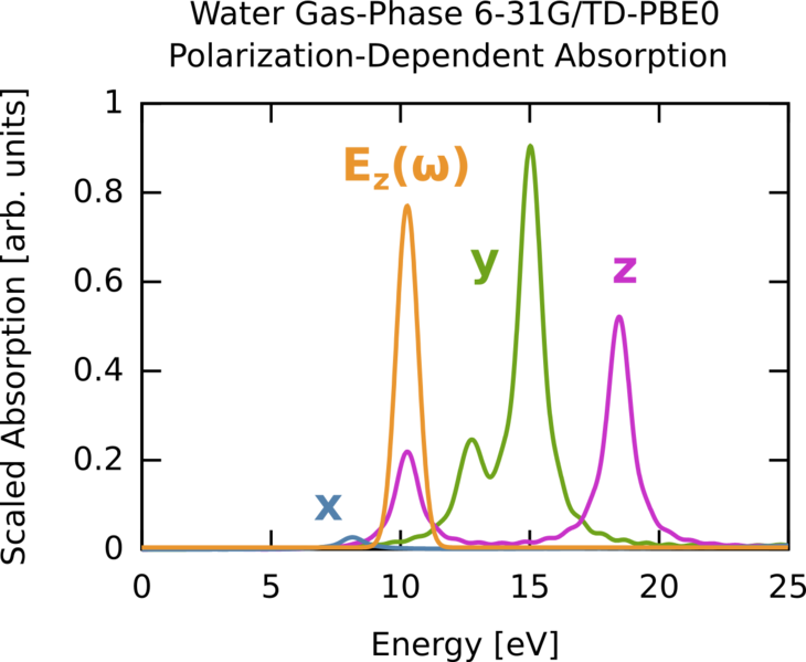
Say we are interested in the excitation near 10 eV. We can clearly see this is a z-polarized transition (green on curve). To selectively excite this we could use a continuous wave E-field, which has a delta-function, i.e., single frequency, bandwidth but since we are doing finite simulations we need a suitable envelope. The broader the envelope in time the narrower the excitation in frequency domain, but of course long simulations become costly so we need to put some thought into the choice of our envelope. In this case the peak of interest is spectrally isolated from other z-polarized peaks, so this is quite straightforward. The procedure is outlined below, and the corresponding frequency extent of the pulse is shown on the absorption figure in orange. Note that it only covers one excitation, i.e., the field selectively excites one mode. The full input deck is h2o_resonant.nw .
The relevant code section is:
rt_tddft
  tmax 1000.0
  dt 0.2

  field "driver"
    type gaussian
    polarization z
    frequency 0.3768  # = 10.25 eV
    center 393.3
    width 64.8
    max 0.0001
  end

  excite "system" with "driver"
 end
task dft rt_tddft
Run now h2_resonant.nw on 4 cores:
bsub -n 4 -o resonant.out mpirun nwchem resonant.nw
The run (follow with bpeek) will apply a field for a limited amount of time. This field will excite the system into a superposition of the ground state and the one excited state, which manifests as monochromatic oscillations. After the field has passed the dipole oscillations continue forever as there is no damping in the system. There are 5000 MD steps. It will take about 10 minutes. At the end, cubefiles for the density at each timestep will be generated. You can visualize the animation using vmd, using a script that cleans a bit (moving the cubes into another directory)
./createlist
vmd -e animate.cube.vmd
What you will see is the electron density difference between the initial state and an instant along the trajectory.
- Plot from the output file the applied field: grep -i Applied resonant.out | grep alpha > appl
- Plot the z component of the induced dipole moment: grep ipole resonant.out > dipole
- Explain what you see in the vmd representation based on what you see on the previous plot