Water molecular models are computational techniques that have been developed in order to help discover the structure of water. In this section, you will be asked to calculate some physical properties based on classical molecular dynamics simulation. The TIP3/Fw model will be used in the simulations.

We have prepared a CP2K input file water.inp for running a MD simulation of liquid water using the force field from the first exercise (parameterized by Praprotnik et al.).

Next, we are going to analyze the trajectories in order to calculate the radial distribution function (rdf, $g(r)$) as a function of the distance $r$.

VMD comes with an extension for exactly this purpose: In the VMD Main window open “Extensions → Analysis” click on “Radial Pair Distribution function $g(r)$”. In the appearing window use “Utilities → Set unit cell dimensions” to let VMD know the size of the periodic simulation box which you used. After that use Selection 1 and 2 to define the atomic types that you want to calculate the rdf for, for example “element H”.

Now, we will calculate the diffusion coefficient which is a proportionality constant between the molar flux due to molecular diffusion and the gradient in the concentration of the species (or the driving force for diffusion) and is defined by: $6D=\lim_{t\to\infty} \ \frac{\delta <r^2(t)>}{\delta t}$

To evaluate this expression, all that is needed is to evaluate the average of the square of the distance that each atom has traveled since the start of the production phase of the dynamics for each point in time during the simulation, and examining the slope of this function in the long time limit. By storing the initial coordinates, it is straightforward to evaluate the square of the traveled distance. However, some care is needed due to the use of periodic boundary conditions: the program stores x, the coordinates, but in many programs, during the dynamics, if any atom has its x, y, or z coordinate become larger than the box size or smaller than zero, it is moved back to the other side of the box. This has the effect of making the raw distance traveled meaningless. Finally, if you take care of the above, the value of D is obtained from the slope, at a long time, of the right-hand side of the above equation (also be careful with the units).

Once again, VMD comes with an extension for exactly this purpose: In the VMD Main window open “Extensions → Analysis” click on “RMSD Trajectory Tool”. In the appearing window use “all” to let VMD know the molecule you want to track. Tick “Plot”, and press “RMSD”. This will plot the RMSD for the water system.

Now, you will compute the vibrational spectrum and dielectric constant of water based on the previous MD simulation. Reference spectra for water are available from Praprotnik et al.. We provide you with a small FORTRAN program which computes the correlation function of the (derivative of) the dipole moment and performs the Fourier transform:

\begin{equation} A(\omega)\propto{\int\langle{\dot{\mu}}({\tau}){\dot{\mu}}(t+{\tau})\rangle_{\tau}e^{-i{\omega}t}d{t}} \ . \label{eq:auto} \end{equation}

The dielectric constant of a system describes its response to an external electric field. If the dipole moment is properly sampled, one can compute the dielectric constant of water, by applying the Kubo Formula. This is valid in the approximation that the response of the system to the time-dependent perturbation (the field) is linear.

The dielectric constant can then be calculated from the dipole moments via: \begin{equation} \epsilon = 1 + \left(\frac{4 \pi}{3 \epsilon_0 V k_B T } \right ) \operatorname{Var}(M) \ , \end{equation}

where $M$ denotes the dipole moment of the entire simulation cell and $\operatorname{Var}(M)$ denotes the variance of the dipole moment of the sampling: \begin{equation} \operatorname{Var}(M) = (\langle M \cdot M\rangle - \langle M\rangle\langle M\rangle ) \ . \end{equation}

To perform this calculation, compile the FORTRAN code, and execute the program:

gfortran cpt_ir_diele.f90 -o cpt_ir_diele.o
./cpt_ir_diele.o < dipole.in

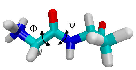
Glyala is one of the simplest molecules that exhibits some important features common to larger biomolecules. In particular, it has more than one long-lived conformation, which we will identify in this exercise by mapping out its potential energy surface.

The conformations of glyala dipeptide are characterized by the dihedral angles of the backbone. Below, we color carbons in green, hydrogens in white, oxygen in red and nitrogen in blue, i.e. the torsional angle $\phi$ is N-C-C-N , while $\psi$ is C-N-C-C along the backbone.

 tar -xvf glyala-epot.tar.gz 

With this knowledge at hand, we will fix the dihedral angles and perform geometry optimization for all remaining degrees of freedom.

Now, we will move to a more realistic system - Glyala in water. We will preformed a MD of glyala in water and save the trajectory.

The initial geometry provided in the PDB file is a glyala molecule solvated by 73 water molecules. The geometry is not equilibrated. You need first to equilibrate the system at 300K. When the system is equilibrated, you need to analysis the result.

 Selection 1, Selection 2 

 element O and not same residue as element C