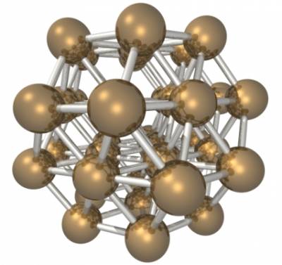
38 atom Lennard-Jones cluster
Download the 1.1 exercise into your EXERCISES folder and unzip it.
max@qmobile:~$ cd ; cd EXERCISES
max@qmobile:~$ wget http://www.cp2k.org/_media/exercises:2018_ethz_mmm:exercise_1.1.zip
max@qmobile:~$ unzip exercises:2018_ethz_mmm:exercise_1.1.zip
max@qmobile:~$ cd exercise_1.1
In this exercise you will test the Lennard-Jones potential. In particular, we will focus on the system described in the following paper about the energy landscape of the 38 atom Lennard-Jones cluster:
The command to run cp2k is the following (with a generic file.inp input file):
max@qmobile:~$ cp2k.ssmp -i file.inp -o file.out
Geometry optimization
In this first part you will perform a simple energy optimization, to find the two lowest lying minima in the potential energy surface.
The input file structure of the template is the following:
- geo_opt.inp
&GLOBAL
 FLUSH_SHOULD_FLUSH
 PRINT_LEVEL low
 PROJECT geo_opt_bfgs
 RUN_TYPE geo_opt
 WALLTIME 600
&END GLOBAL

&MOTION
 &GEO_OPT
  OPTIMIZER BFGS
  MAX_ITER  200
  MAX_DR    0.001
  RMS_DR    0.0003
  MAX_FORCE 0.0001
  RMS_FORCE 0.00003
  &BFGS
   USE_MODEL_HESSIAN yes
  &END BFGS
 &END GEO_OPT
 &PRINT
  &TRAJECTORY on
   FORMAT xyz
   &EACH
    GEO_OPT 1
   &END EACH
  &END TRAJECTORY
 &END PRINT
&END MOTION

&FORCE_EVAL
 METHOD Fist
 STRESS_TENSOR ANALYTICAL
 &MM
    &FORCEFIELD
      &CHARGE
        ATOM Ar
        CHARGE 0.0
      &END
      &NONBONDED
        &LENNARD-JONES
          atoms Ar Ar
          EPSILON 119.8
          SIGMA 3.405
          RCUT 8.4
        &END LENNARD-JONES
      &END NONBONDED
      &CHARGE
        ATOM Kr
        CHARGE 0.0
      &END CHARGE
    &END FORCEFIELD
  &POISSON
   PERIODIC NONE
   &EWALD
    EWALD_TYPE none
   &END EWALD
  &END POISSON
  &PRINT
   &FF_INFO OFF
    SPLINE_DATA
    SPLINE_INFO
   &END FF_INFO
  &END PRINT
 &END MM
 &PRINT
  &FORCES off
  &END FORCES
  &GRID_INFORMATION
  &END GRID_INFORMATION
  &PROGRAM_RUN_INFO
   &EACH
    GEO_OPT 1
   &END EACH
  &END PROGRAM_RUN_INFO
  &STRESS_TENSOR
   &EACH
    GEO_OPT 1
   &END EACH
  &END STRESS_TENSOR
 &END PRINT
 &SUBSYS
  &CELL
   A      100 0 0
   B      0   100 0
   C      0 0 100
   PERIODIC NONE
  &END CELL
  &TOPOLOGY
      COORD_FILE_NAME in.xyz
      COORDINATE xyz
  &END
  &PRINT
   &CELL
   &END CELL
   &KINDS
   &END KINDS
   &MOLECULES OFF
   &END MOLECULES
   &SYMMETRY
   &END SYMMETRY
  &END PRINT
 &END SUBSYS
&END FORCE_EVAL
1 Kelvin*K_b=3.2E-6 Hartree
. Using this conversion factor you can transform the epsilon value into Hartree, and the total energy can be expressed in units of epsilon. The sigma value is in Angstrom.
- randomize the coordinate files fcc.xyz (which represents the “cubic” structure)
m_xyzrand 1.0 < fcc.xyz > fcc_rand.xyz
Do the same with ico.xyz which represents the icosahedral structure. You can look at all files with vmd.
- extract the q4 order parameter from fcc.xyz and from fcc_rand.xyz and compare the values.
python stein.py file.xyz
You will be asked the cutoff radius for the neighbors, it is 1.391 in sigma units. You should input it in Angstrom. You will also be asked “value of l” This means the symmetry of the order parameter, which is l=4 in this case.
- before running the simulation, copy the input coordinate file into in.xyz
cp fcc_rand.xyz in.xyz
- Before running cp2k, check if the file OPT-pos-1.xyz is already present from a previous run. In that case remove or delete it accordingly. It contains the trajectory of the optimization.
- run cp2k
cp2k.ssmp -i geo_opt.inp | tee geo_opt.out
(to see the output on the screen as well), or AS AN ALTERNATIVE
cp2k.ssmp -i geo_opt.inp > geo_opt.out
(to retain the output in the geo_opt.out file only)
- in the output file, grep the final energy
grep "ENERGY|“ geo_opt.out
and transform it in the unit of the paper (epsilon units)
- Open vmd and play with the optimization trajectory
vmd OPT-pos-1.xyz
(ask the teacher)
- apply the script myq4 to the optimization trajectory: this generates a list of q4 and energies for the whole trajectory.
./myq4 OPT-pos-1.xyz > fcc.ene.q4
- plot q4 and energies with gnuplot (ask the teacher)
- have a look at the myq4 script
nano myq4
- repeat for the ico.xyz starting point, don't forget to first copy/remove the files appropriately. For example:
mkdir FCC ; mv OPT* FCC ; mv geo_opt.out FCC
- Run the bash script
./curve
Look inside, and try to understand what you get.
- create a FCC_OUT subdirectory (mkdir FCC_OUT ; cd FCC_OUT) and copy there the files you want to keep; then go back one dir (cd ..), delete all the OPT* files (rm OPT* ) and repeat the exercise with ico.xyz
- Report the energy of the minima, compare it with the ones of the initial configurations.
- After converting the energy into “epsilon” units, estimate the number of bonds in the cluster, assuming a pairwise interaction.
- Plot q4 vs. energy and q4 vs. optimization steps, for the two cases. Discuss the results. Are the minima in two separate basins?
- Report the value of the order parameter of the minumum, and discuss what you see
- Use “gnuplot” to make the output of “./curve” understandable, discuss the results.

